EAGLE-4: Notes on the Efficient LM Head and Earlier Experiments

English translation of my original article on Zhihu.

Following the release of EAGLE-4, I wanted to share a former EAGLE Team member’s perspective on its design, drawing on the technical report and some of the experiments and tradeoffs I was involved in.

For context, I was a member of the EAGLE Team from August 2025 to June 2026. I later joined LongCat, and I now work on MTP and speculative decoding optimizations at Kimi. The two-stage design of the EAGLE Efficient LM Head and its training-free version were work I designed and validated while on the team. They are the main focus of this retrospective.

The technical report focuses on EAGLE-Harness and the EAGLE Efficient LM Head. I will briefly discuss the Harness first, then go into the LM Head, which I know better.

EAGLE-Harness

EAGLE-Harness is a set of dynamic speculative decoding components integrated with SGLang and vLLM, similar in spirit to DSpark’s dynamic verification logic. It uses factors such as draft and target costs and draft confidence to construct a draft tree dynamically, then sends that tree to the target model for verification. The main differences from DSpark’s dynamic verification are:

• Early stopping during drafting. DSpark mainly selects a prefix of an already generated draft block for verification. Because EAGLE drafts autoregressively, EAGLE-Harness also considers stopping the draft process early. If the expected benefit of another drafting step does not justify its additional cost, drafting can stop before reaching the preset maximum depth.
• Support for draft trees. Both early stopping and pruning before verification can operate on a draft tree. DSpark’s dynamic verification scheme is designed for chains.
• A different estimate of the expected accepted-token count. EAGLE-Harness reuses draft probabilities with some heuristics, rather than requiring a separately trained confidence head. DSpark relies on a dedicated confidence head. I will leave the details of the Harness heuristics aside here.

It is natural to see EAGLE-Harness as a follow-up to a “DSpark-Harness.” From what I knew while on the team, however, its prototype came from former colleague Yinrong Hong and others’ CAST. That paper was posted on arXiv in October 2025. Even accounting for later optimizations, the approach was already quite mature by early 2026.

EAGLE Efficient LM Head

The Efficient LM Head was a design I developed and validated while on the team. Here is some of the reasoning behind it.

By late 2025, it was already clear that the draft model’s LM Head was expensive. For a one-layer draft model such as EAGLE, the LM Head alone could account for roughly half of the draft forward-pass time in some configurations.

The common solution at the time, used by methods such as FR-Spec, was vocabulary pruning: remove infrequent tokens and retain a smaller, fixed vocabulary. EAGLE-3 also adopted this approach, typically reducing the vocabulary to 32,000 tokens.

In later experiments, however, restoring the full vocabulary from 32,000 tokens increased the acceptance length by about one token. That was a substantial gain in our tests. Vocabulary pruning saved LM Head computation, but it also noticeably reduced the drafter’s predictive ability.

Could we retain the acceptance length of the full vocabulary while reducing the LM Head’s cost? I mainly explored three directions:

1. Make the LM Head computation cheaper directly, through low-rank approximation, quantization, or similar techniques, and use the approximate logits as the output.
2. Use a two-stage method at the token level. First select candidates with a cheap method, then use the full LM Head to compute logits only for those candidates.
3. Use a two-stage method at the cluster level. Group tokens into clusters, for example 128 tokens each. First select a few clusters, then compute logits for all tokens in those clusters and sample from them. Google’s Gemma 4 later used a similar idea.

We chose the second approach. In the configurations we tested, it was the only one that preserved almost all of the acceptance length of the full LM Head. The first approach lost a substantial amount of acceptance length, and the third also showed a noticeable loss.

For the first-stage selector, we tried low-rank approximation, quantization, and combinations of the two. After considering the tradeoffs, we settled on a purely low-rank approach without quantization.

This led to the basic design of the EAGLE Efficient LM Head:

• Stage one: use a low-rank head to score the full vocabulary cheaply, then select candidates with Top-$k$.
• Stage two: gather the full LM Head rows corresponding to those candidates and recompute their logits using the original hidden states.

The computational pattern resembles DSA: use a cheap module to select a subset, then perform the full computation on that subset.

Here is a sketch I made at the time:

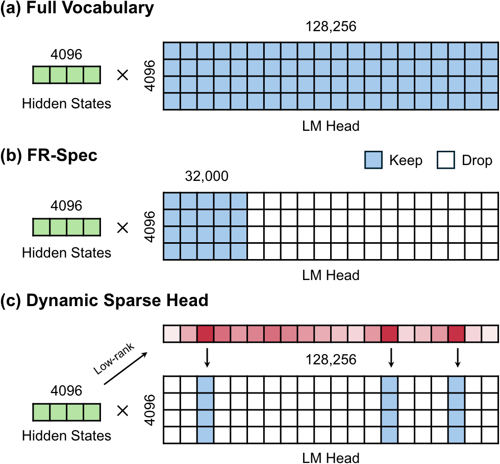
At this point, the idea is hardly unusual. For example, SpecVocab, released in February 2026, proposed an almost identical computational pipeline. Still, our two-stage approach had largely taken shape by December 2025.

A training-free version: frequency-aware SVD

Our earliest version differed from the one in the current technical report: it did not require additional training of the low-rank head. I called it frequency-aware SVD, or Freq-aware SVD: truncated SVD that accounts for token frequency.

The intuition is simple. Ordinary truncated SVD does not distinguish between LM Head rows for frequent tokens and those for rare tokens. With a limited rank, we would prefer to allocate more approximation accuracy to frequent tokens, since they appear more often during generation.

Concretely, we weight each row of the LM Head by token frequency, perform truncated SVD, then undo the row scaling. Inference still approximates the original LM Head; we do not multiply the output logits by token frequencies.

Let the full LM Head be $W \in \mathbb{R}^{n \times d}$ and the frequency-weight matrix be $F = \operatorname{diag}(f_1,\ldots,f_n)$. The low-rank factors $A$ and $B$ are computed as:

Here, $U_r$, $\Sigma_r$, and $V_r$ retain the top $r$ singular values and their corresponding vectors. The frequency weights need smoothing so that every $f_i > 0$.

This gives the low-rank head used to screen candidates. Given a hidden state $h$, compute $A(Bh)$ and take the Top-$k$. Apart from collecting token frequencies and performing one decomposition, no additional training is needed. Although the paper does not discuss this version, the public code still contains the corresponding implementation.

Interestingly, this training-free approach was still the version we used when I left the team. In the models and configurations we tested, it already preserved almost all of the acceptance length. We also tried some simple training-based strategies, including training after SVD initialization, but they either matched or underperformed the training-free version. At the time, that gave us little incentive to keep pursuing them.

The EAGLE-4 report shows that the later version does benefit from training the low-rank candidate head. Its approach freezes the rest of the drafter and trains only the two low-rank factors. That was a later development.

A variant based on local Top-k

We also tried a more efficient variant.

The two-stage design reduced the matrix multiplication cost, but stage one still wrote approximate scores for the full vocabulary to HBM and then read them back for a global Top-$k$. This was also a significant cost in our implementation.

The original pipeline looked roughly like this:

u = B @ h
scores = A @ u                 # Write full-vocabulary scores to HBM.
ids = topk(scores, C).indices   # Read them back for a global Top-k.
logits = W[ids] @ h

We therefore replaced global Top-$k$ with local Top-$k$, fused directly into the matrix multiplication tiles:

u = B @ h

# Conceptual pseudocode: each GPU program handles one vocabulary tile.
parallel_for tile in vocab_tiles:
    scores = A[tile] @ u       # Finish rank reduction; keep scores on-chip.
    local_ids = topk(scores, k_tile).indices
    store(candidate_ids[tile], tile.token_ids[local_ids])

ids = concat(candidate_ids)   # About number_of_tiles * k_tile candidates.
logits = W[ids] @ h

This resembles Google’s bucketed approximate Top-$k$: fuse local selection with matrix multiplication. Each tile retains only a small number of candidates and writes out their token indices. The candidates from all tiles are then combined and passed to the full LM Head for exact recomputation in stage two. This avoids both the HBM write of all approximate scores and the subsequent global Top-$k$ over those scores.

Local Top-$k$ does not guarantee the same candidate set as global Top-$k$. If many important tokens fall in the same tile, for example, some may be excluded by that tile’s candidate quota. In our tests, however, the acceptance-length loss was usually within 0.05 tokens.

One small but useful detail: shuffle the vocabulary rows before applying local Top-$k$. We observed that tiling the vocabulary in its original order hurt candidate recall; shuffling the rows before tiling improved it substantially. Graphcore’s work also discusses random permutations as a way to improve recall.

EAGLE-3.1

I also want to briefly discuss EAGLE-3.1. EAGLE-4 inherits two normalization changes from it: FC Norm and Post-norm.

FC Norm applies RMSNorm separately to the hidden states extracted from several target-model layers, before concatenating them and passing them through the fully connected projection.

Former colleague Haochen Gu and I found this useful while training a GPT-OSS drafter. We noticed that the target hidden states produced very large hidden-state norms after the FC projection, so we tried adding normalization before it. In those experiments, this led to faster convergence and improved training accuracy by about two percentage points, so we kept it.

After EAGLE-3.1 was released, I heard comments that FC Norm did not really help. We had seen that too: its benefits are model-dependent. In our experiments, it helped GPT-OSS, while the difference was much less apparent for some other models.

We did not observe degradation from adding it, so my personal preference was to keep it: some models gained a little, while others were roughly unchanged. That is only an observation from the configurations we tested, of course, not a general claim that adding it can never hurt.

Post-norm passes the hidden states after the output RMSNorm to the next draft step, preventing unnormalized hidden states from accumulating larger norms during recurrence. I did not work on this part. The Attention Drift paper discusses it in detail, so I will leave it there.

A few closing thoughts

If EAGLE-Harness and the Efficient LM Head had already taken shape so much earlier, why were they only released now?

From my experience while on the team, there was not much pressure to publish. Most of our effort went into improving EAGLE, and we were in no particular hurry to write a paper or publicize the work. This describes the period when I was there; it should not be taken as an explanation of the entire later release process.

We also explored other interesting designs that do not appear in this technical report. Since those remain unpublished, I will not discuss them here.