DFlash-2's Selector and DSpark's Markov Head: An Equivalence Observation

English translation of my original article on Zhihu.

When DFlash-2 was released, many readers viewed its Selector as a new calibration method distinct from DSpark’s Markov Head. A closer look reveals a strong connection: remove the hidden-state term from the Selector, and the two become identical in matrix form. Following this equivalence also leads to two interesting implications. This post records that observation.

The main points are:

• The Selector and the Markov Head share the same mechanism: base logits plus a low-rank token-transition bias. Without the hidden-state gate $H(h_t)$, their formulas are identical, and both use a 256-dimensional factorization.
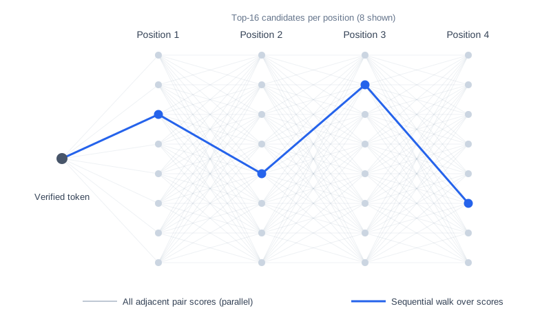
• The Selector’s parallelism comes from restricting calibration to top-16 candidate sets. It precomputes calibrated logits for every adjacent candidate pair in parallel, leaving only a lightweight sequential walk.
• Two implications follow: DFlash-2 can be trained in a DSpark-style formulation without treating the Selector as a separate mechanism; an already trained DSpark model can use the same top-$k$ truncation to parallelize calibration without retraining.

What the two methods do

DSpark’s Markov Head. A parallel backbone computes the base logits $U_k$ for the entire block in one pass. To introduce dependencies between neighboring tokens, DSpark adds a small sequential module: after sampling a token, it uses that token to add a bias vector to the logits at the next position:

\[\begin{gathered} \operatorname{logits}_k = U_k + W_1[a]^\top W_2, \\ W_1 \in \mathbb{R}^{V \times 256},\quad W_2 \in \mathbb{R}^{256 \times V}. \end{gathered}\]

Here, $a$ is the previously sampled token, $W_1[a]$ is its 256-dimensional embedding, and $W_1[a]^\top W_2$ is a bias vector over the full vocabulary.

DFlash-2’s Selector. At each position, it retains the top-16 candidates and scores all pairs of candidates at adjacent positions:

\[S_t(a,b) = U_t(b) + \left\langle A(a) \odot H(h_t),\ B(b) \right\rangle.\]

Both $A$ and $B$ assign a 256-dimensional embedding to each token. The context-dependent gate $H(h_t)$ is computed from the current hidden state.

The equivalence: remove the gate, recover the Markov Head

First, write DSpark’s bias vector $W_1[a]^\top W_2$ for a single candidate $b$. This gives $W_1[a]^\top W_2[:,b]$: the inner product between $W_1[a]$ and column $b$ of $W_2$.

\[\operatorname{logits}_k(b \mid a) = U_k(b) + W_1[a]^\top W_2[:,b].\]

In words: a base logit plus the inner product of the previous token’s embedding and the current candidate’s 256-dimensional vector.

Now remove $H(h_t)$ from the Selector, or equivalently set it to the all-ones vector. Its score becomes:

\[S_t(a,b) = U_t(b) + A[a]^\top B[b].\]

Putting the two side by side:

\[\begin{gathered} \text{DSpark:} \\ \operatorname{logits}_k(b \mid a) = U_k(b) + W_1[a]^\top W_2[:,b], \\[8pt] \text{DFlash-2 without gating:} \\ S_t(a,b) = U_t(b) + A[a]^\top B[b]. \end{gathered}\]

The formulas are identical: a base logit plus an inner product between two 256-dimensional vectors. The correspondence is $W_1[a] \leftrightarrow A[a]$ and $W_2[:,b] \leftrightarrow B[b]$.

The only extra term is $H(h_t)$. With the gate retained, the Selector is equivalent to the following DSpark-style calibration rule, which can be viewed as a context-gated variant of the Markov Head:

\[\operatorname{logits}_t = U_t + \bigl(W_1[a] \odot H(h_t)\bigr)^\top W_2.\]

Where the parallelism comes from

The Selector and the Markov Head are fundamentally the same kind of probability calibration. Yet DSpark appears to require sequential execution: the previous token must be sampled before the next position’s logits can be calibrated. The causal dependency seems unavoidable.

What lets the Selector parallelize this computation? Essentially, two choices:

1. Fix the candidate sets. At each position, retain only the top-16 tokens under the base logits. Each step must choose from that fixed set of 16 candidates.
2. Precompute every calibration within those sets. For each pair of adjacent positions, compute the calibrated logits for all $16 \times 16$ possible predecessor–candidate pairs in parallel.

Instead of waiting for the previous token before computing the calibration, we compute all possibilities in advance and look up the appropriate scores once that token is known. The remaining sequential work is a greedy walk, or sampling, over the precomputed scores, which is inexpensive.

Two implications

1. Train DFlash-2 using the equivalent Markov Head formulation

Consider the gated DSpark-style module:

\[\operatorname{logits}_t = U_t + \bigl(W_1[a] \odot H(h_t)\bigr)^\top W_2.\]

Because this is equivalent to the Selector’s scoring formula, we do not need to treat the Selector as a separate concept when expressing the training computation. We can train a DSpark-style module using this formula, then, at inference time, fix the top-16 candidate sets, compute all within-set calibrations in parallel, and perform the walk. This recovers the Selector’s computation.

In other words: DFlash-2’s Selector = a gated DSpark-style Markov Head + top-16 parallel execution.

2. Parallelize DSpark’s candidate calibration without retraining

Conversely, an already trained DSpark model can use the same execution strategy without retraining, by restricting calibration to the top-$k$ tokens of the base distribution:

1. Use the parallel backbone to obtain the top-$k$ candidates at each position.
2. For every pair of adjacent positions, precompute the calibrated logits for all $k \times k$ candidate pairs in parallel: the base logit plus the transition bias.
3. Perform a lightweight sequential walk over those scores, with rejection sampling preserving the target output distribution.

References

• DFlash 2: Keep Drafting Parallel
• DSpark: Confidence-Scheduled Speculative Decoding with Semi-Autoregressive Generation